Step 1: Material model

The first step to perform a CRATE simulation is to generate a suitable computational model that characterizes the microstructure of the heterogeneous material under analysis.

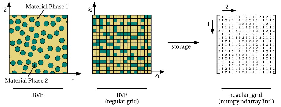
Attending to the concepts introduced here, such a computational model is named Representative Volume Element (RVE) and can be obtained in two different ways:

• Experimentally. Through a suitable microstructure imaging method (e.g., two-dimensional scanning electron microscopy (SEM), three-dimensional micro-computed tomography (\({\mu}\) CT));

• Computationally. Adopting a suitable computational generation method (e.g., AMINO for particle-reinforced materials, NEPER for polycrystalline materials).

Note

The generation of the RVE is not part of CRATE!

---

CRATE accepts any kind of RVE that satisfies the following requirements:

• Requirement 1: The RVE must be quadrilateral (2d) or paralelepipedic (3d);

• Requirement 2: The RVE must be spatially discretized in a regular grid of voxels, where each voxel is associated with a given material phase as illustrated below:

• Requirement 3: The RVE spatial discretization file (.rgmsh file) that is ultimately provided to CRATE as part of the input data must be generated with NumPy as demonstrated and explained in the following Python (pseudo-)script:

  # python_script.py
  
  # The RVE discretization in a regular grid of voxels (2d or 3d), where each voxel
  # is associated with a given material phase, must be materialized as a NumPy ndarray
  # (2d or 3d), where each entry corresponds to a given voxel. Hence, each entry of the
  # ndarray contains the identifier (integer) of the corresponding voxel's material phase.
  # Assume that the ndarray is called `regular_grid`.
  regular_grid = ...
  
  # The spatial discretization file (.rgmsh) is then generated by saving the `regular_grid`
  # ndarray in binary format through the NumPy save function. Note that this appends the
  # .npy extension to the filename.
  np.save('example_rve.rgmsh', regular_grid)
  
  # Output: example_rve.rgmsh.npy file